Blogs and Learning Notes

GRPO（Group Relative Policy Optimization）理解

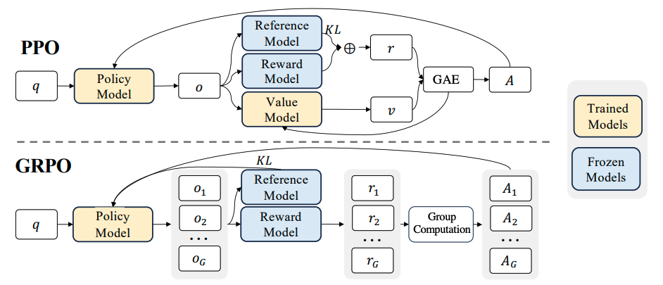
GRPO的核心思想可以简要理解为Grouped PPO。

也就是说，对同一个问题$q$, 一次性采样一组（$G$ 个）完整回答，用组内相对优势（而不是 value baseline）来做 PPO-style 的 token 级策略更新，同时用KL正则把策略约束在参考模型附近。

这里的Group指的就是分组；Relative指的就是组内相对优势。

GRPO示意图

接下来，我想根据GRPO中涉及到的公式，和对应的伪代码，深入理解一下GRPO里面的细节；如果你对公式不感兴趣，那么可以直接跳过公式回顾和深入理解的部分。

公式回顾

原文中公式如下：

\[\begin{aligned} \mathcal{J}_{G R P O}(\theta) & =\mathbb{E}_{\left[q \sim P(Q),\left\{o_i\right\}_{i=1}^G \sim \pi_{\theta_{o l d}}(O \mid q)\right]} \\ & \frac{1}{G} \sum_{i=1}^G \frac{1}{\left|o_i\right|} \sum_{t=1}^{\left|o_i\right|}\left\{\min \left[\frac{\pi_\theta\left(o_{i, t} \mid q, o_{i,<t}\right)}{\pi_{\theta_{o l d}}\left(o_{i, t} \mid q, o_{i,<t}\right)} \hat{A}_{i, t}, \operatorname{clip}\left(\frac{\pi_\theta\left(o_{i, t} \mid q, o_{i,<t}\right)}{\pi_{\theta_{o l d}}\left(o_{i, t} \mid q, o_{i,<t}\right)}, 1-\varepsilon, 1+\varepsilon\right) \hat{A}_{i, t}\right]-\beta \mathbb{D}_{K L}\left[\pi_\theta| | \pi_{r e f}\right]\right\} \end{aligned} % \tag{1}\]

我感觉作者省略了一对括号，对数学不好的同学不太友好，因此这里给它加上，长成这样：

\[\begin{aligned} \mathcal{J}_{\text{GRPO}}(\theta) &= \mathbb{E}_{\left[q \sim P(Q), \{o_i\}_{i=1}^G \sim \pi_{\theta_{\text{old}}}(o|q)\right]} \Bigg[ \frac{1}{G} \sum_{i=1}^G \frac{1}{|o_i|} \sum_{t=1}^{|o_i|} \Bigg\{ \min \Bigg[ \frac{\pi_\theta(o_{i,t}\mid q, o_{i,<t})} {\pi_{\theta_{\text{old}}}(o_{i,t}\mid q, o_{i,<t})} \hat{A}_{i,t}, \\ &\quad\quad \operatorname{clip}\!\left( \frac{\pi_\theta(o_{i,t}\mid q, o_{i,<t})} {\pi_{\theta_{\text{old}}}(o_{i,t}\mid q, o_{i,<t})}, 1-\varepsilon, 1+\varepsilon \right) \hat{A}_{i,t} \Bigg] - \beta \, D_{\text{KL}}\!\left[\pi_\theta \,\|\, \pi_{\text{ref}}\right] \Bigg\} \Bigg] \end{aligned}\]

整个 GRPO 目标函数 $\mathcal{J}{\text{GRPO}}(\theta)$ 是一个期望收益（expected objective），即模型策略 $\pi\theta$在大量不同任务（prompts）和生成结果(responses)上的整体表现水平（由 group-normalized advantage 加权，并减去 KL 正则项表示）。

因此，我们的目标是：通过调整 $\theta$，让这个期望收益尽可能大。

注：在实际训练中，为了兼容基于梯度下降的优化框架，通常做法是最小化其负值，即定义： \(\mathcal{L}_{\text{GRPO}}(\theta) = -\mathcal{J}_{\text{GRPO}}(\theta)\) 并对 $\mathcal{L}_{\text{GRPO}}(\theta)$ 执行梯度下降。

深入理解

1. 最外层期望（Expectation）：在什么分布上进行优化？

\[\mathbb{E}_{[q \sim P(Q), \{o_i\}_{i=1}^G \sim \pi_{\theta_{\text{old}}}(o|q)]}\]

其中, $q$表示一个 prompt（问题），从数据分布 $P(Q)$ 中采样， $P(Q)$包含了不同类型的prompt，例如医学问题，VQA、报告生成等； ${o_i}{i=1}^G$表示对同一个 $q$，用旧策略 $\pi{\theta_{\text{old}}}$ 生成的 G 个输出（completions）. 也就是说：对每个 prompt，我们并行生成 G 个回答，然后基于这些回答做优化. 这就是 GRPO 的“组内对比”思想.

进一步理解，这个期望可以表示：”如果我们从真实 prompt 分布中随机挑一个 $q$，再用旧策略对它生成 $G$ 个随机回答，然后计算 GRPO loss，那么这个 loss 的平均值是多少?”，而我们的目标是：通过调整 $\theta$（当前策略），让这个期望 loss 尽可能小。”

这里我们通过监督学习来做个类比，监督学习的目标函数如下：

\[\mathcal{L}(\theta) = \mathbb{E}_{(x, y) \sim \mathcal{D}} \left[ \text{CrossEntropy}(f_\theta(x), y) \right]\]

其中$\mathcal{D}$表示训练数据分布，$(x, y)$表示一条样本（如图像+标签），CrossEntropy表示对这条样本计算的 loss。那么这个公式的整体含义可以表示为：在所有可能的数据上，模型预测的平均交叉熵损失。

但我们无法计算真实期望（因为 $\mathcal{D}$ 未知），所以用 Monte Carlo 估计（即 mini-batch）：

\[\hat{\mathcal{L}}(\theta) \approx \frac{1}{N} \sum_{i=1}^N \text{CrossEntropy}(f_\theta(x_i), y_i)\]

也就是说，期望 = 理论目标，求和 = 实际近似。回到 GRPO,完全一样的逻辑,对应关系如下：

监督学习	GRPO
数据分布 $\mathcal{D}$	Prompt 分布 $P(Q)$ + 旧策略生成分布 $\pi_{\theta_{\text{old}}}$
一条样本 $(x, y)$	一组数据 $(q, o_1, …, o_G)$
Loss 函数（如 CE）	PPO-style clipped objective + KL penalty
期望 $\mathbb{E}_{(x,y)\sim\mathcal{D}}[\text{loss}]$	$\mathbb{E}_{q, {o_i}}[\text{GRPO loss}]$

2. 分组平均 && Token平均：保持梯度稳定的同时拉齐不同序列长度的贡献

从下面的公式，可以看到这里有两层平均，外层平均表示对一个prompt产生的分组内部loss做平均，避免$G$变大导致梯度爆炸；内层对token再平均，使得不同长度的回答被归一化到相同的尺度，防止模型生成更长的token来刷reward。

\[\frac{1}{G} \sum_{i=1}^G \frac{1}{|o_i|} \sum_{t=1}^{|o_i|} \left\{ \cdots \right\}\]

具体地，对于每个 output $o_i$：计算其每个 token $t$ 对应的 loss，其中$|o_i|$表示$o_i$的序列长度； 然后对所有 token 取平均（$\frac{1}{|o_i|}$）； 再对所有 G 个 output 取平均（$\frac{1}{G}$）。

3. PPO-style Clipped Objective

接下来我们看一下大括号内部，实际上是新旧策略之间的token级重要性采样比(Importance Sampling Ration, ISR)和优势值(Advantage)的乘积，具体地：

\[\min \left[ \frac{\pi_\theta(o_{i,t}|q, o_{i,<t})}{\pi_{\theta_{\text{old}}}(o_{i,t}|q, o_{i,<t})} \hat{A}_{i,t}, \, \text{clip}\left( \frac{\pi_\theta(o_{i,t}|q, o_{i,<t})}{\pi_{\theta_{\text{old}}}(o_{i,t}|q, o_{i,<t})}, 1-\varepsilon, 1+\varepsilon \right) \hat{A}_{i,t} \right]\]

其中，$\pi_{\theta}$表示当前待优化的策略模型（policy）， $\frac{\pi_\theta}{\pi_{\text{old}}}$为ISR， $o_{i,t}$表示第 $i$ 个回答的第 $t$ 个 token， $o_{i,<t}$表示第 $i$ 个回答中第 $t$ 个 token 之前的前缀； $\hat{A}_{i,t}$表示第 $i$ 个 output 中第 $t$ 个 token 的优势值； clip(...)限制了ISR 在 $[1-\varepsilon, 1+\varepsilon]$ 范围内，防止策略更新过大； 最终取 min，这是标准PPO 损失，用于稳定训练。

接下来，我们还需要重点说明的是优势值的计算。$\hat{A}_{i,t}$的计算方式如下： 对每个 output $o_i$，先计算其总 reward $r_i$（如 accuracy、LLM judge 分数）； 然后对组内 reward 做标准化：

\[\hat{A}_i = \frac{r_i - \mu_r}{\sigma_r + \epsilon}\]

最后将 $\hat{A}i$ 广播到该 output 的所有 token 上（即 $\hat{A}{i,t} = \hat{A}_i$）。这里$\epsilon$用于保持数值稳定。

4. KL 正则项（对齐 && 防止遗忘）

\[- \beta D_{\text{KL}}[\pi_\theta \| \pi_{\text{ref}}]\]

其中，$D_{\text{KL}}[\pi_\theta | \pi_{\text{ref}}]$表示当前策略与参考模型（通常是 SFT 模型）之间的 KL 散度；$\beta$为超参数，控制正则强度；减号表示：我们希望最小化这个 KL，即不让新策略偏离参考模型太远。最后，让我们看一下GRPO原文中对KL散度的定义：

\[\mathcal{D}_{KL}\left[\pi_\theta \mid\mid \pi_{\text{ref}}\right] = \frac{\pi_{\text{ref}}(o_{i,t} \mid q, o_{i,<t})}{\pi_\theta(o_{i,t} \mid q, o_{i,<t})} - \log \frac{\pi_{\text{ref}}(o_{i,t} \mid q, o_{i,<t})}{\pi_\theta(o_{i,t} \mid q, o_{i,<t})} - 1\]

伪代码

原始论文中算法流程：

GRPO伪代码

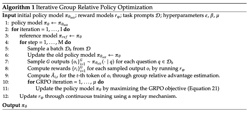
下面是我从ms-swift文档中摘抄的GRPO的伪代码，供大家理解。这里可以看到，代码中会在原始公式的整体加上负号，以最小化损失函数。

# ========== 1. Rollout Generation Phase ==========
prompt = "Question: Which is bigger? 9.11 or 9.9?"

# Generate multiple completions through parallel sampling
completions = rollout_function(
    model=current_policy_model,
    prompt=prompt,
    num_generations=8,  # Hyperparameter: number of samples per prompt
    temperature=1.0     # Hyperparameter: sampling diversity
)
"""
completions = [
    (completion 1) "The larger number is 9.11...",
    (completion 2) "9.9 is bigger than...",
    ...
    (completion 8) "After calculation, 9.11..."
]
"""

# ========== 2. Reward Calculation Phase ==========
# Evaluate generated completions using reward model
rewards = reward_function(
    completions=completions,
    ground_truth="9.11"  # Expected correct answer
)
"""
rewards = [
    (reward 1) 1.0,  # Correct answer
    (reward 2) 0.0,  # Incorrect
    ...
    (reward 8) 1.0   # Correct
]
"""

# Normalize rewards to advantages
rewards_mean = mean(rewards)  # μ = 0.5
rewards_std = std(rewards)    # σ = 0.25
advantages = (rewards - rewards_mean) / (rewards_std + 1e-8)  # Standardization
"""
advantages = [
    (advantage 1)  2.0,  # (1.0 - 0.5)/0.25
    (advantage 2) -2.0,
    ...
    (advantage 8)  2.0
]
"""

# ========== 3. Policy Optimization Phase ==========
# Get token-level log probabilities from different models
current_logps = get_per_token_logps(current_policy_model, prompt, completions)  # π_θ
old_logps = get_per_token_logps(old_policy_model, prompt, completions)          # π_θ_old
ref_logps = get_per_token_logps(reference_model, prompt, completions)           # π_ref

# PPO Clipped Objective
is_ratio = exp(current_logps - old_logps)  # Importance sampling ratio: e^(π_θ - π_θ_old)
clipped_ratio = clip(is_ratio, 1-ε, 1+ε)   # ε=0.2 typically

# Policy gradient term (dual form)
policy_loss = -mean(
    minimum(is_ratio * advantages,       # Unclipped objective
           clipped_ratio * advantages)  # Clipped objective
)

# KL Divergence Penalty (K3 estimator)
# KL(π_θ||π_ref) ≈ e^(logπ_ref - logπ_θ) - (logπ_ref - logπ_θ) - 1
kl_penalty = beta * mean(
    exp(ref_logps - current_logps) -
    (ref_logps - current_logps) - 1
)

# Total Loss = Policy Loss + KL Penalty
total_loss = policy_loss + kl_penalty

# ========== 4. Update Rule ==========
# Apply gradient descent to minimize total_loss
optimizer.zero_grad()
total_loss.backward()
optimizer.step()

参考资料

[1]. DeepSeekMath: Pushing the Limits of Mathematical Reasoning in Open Language Models

[2]. https://swift.readthedocs.io/zh-cn/latest/Instruction/GRPO/GetStarted/GRPO.html

[3]. Qwen & ChatGPT

This site is open source. Improve this page.